Raw data visualization using Python
This notebook shows how to visualize the raw data in my paper using Python 3. The raw data basically refers to unprocessed results directly coming from the surface integral equation (SIE) computation, but it also includes input parameter sets and simulation mesh to help understand the simulation itself.
The raw data consists of various types of data:
- Input parameter sets for calculation:
.xmlfiles - Simulation mesh:
.meshfiles - Raw data directly from the computation:
.solfiles containing a huge array of numbers (surface currents) - Semi-processed data having physical meaning:
.ein,.esc,.hin,.hscfiles for electric and magnetic field amplitudes
The files are located in the RawData folder and grouped into subfolders for different simulations.
0. Data structure
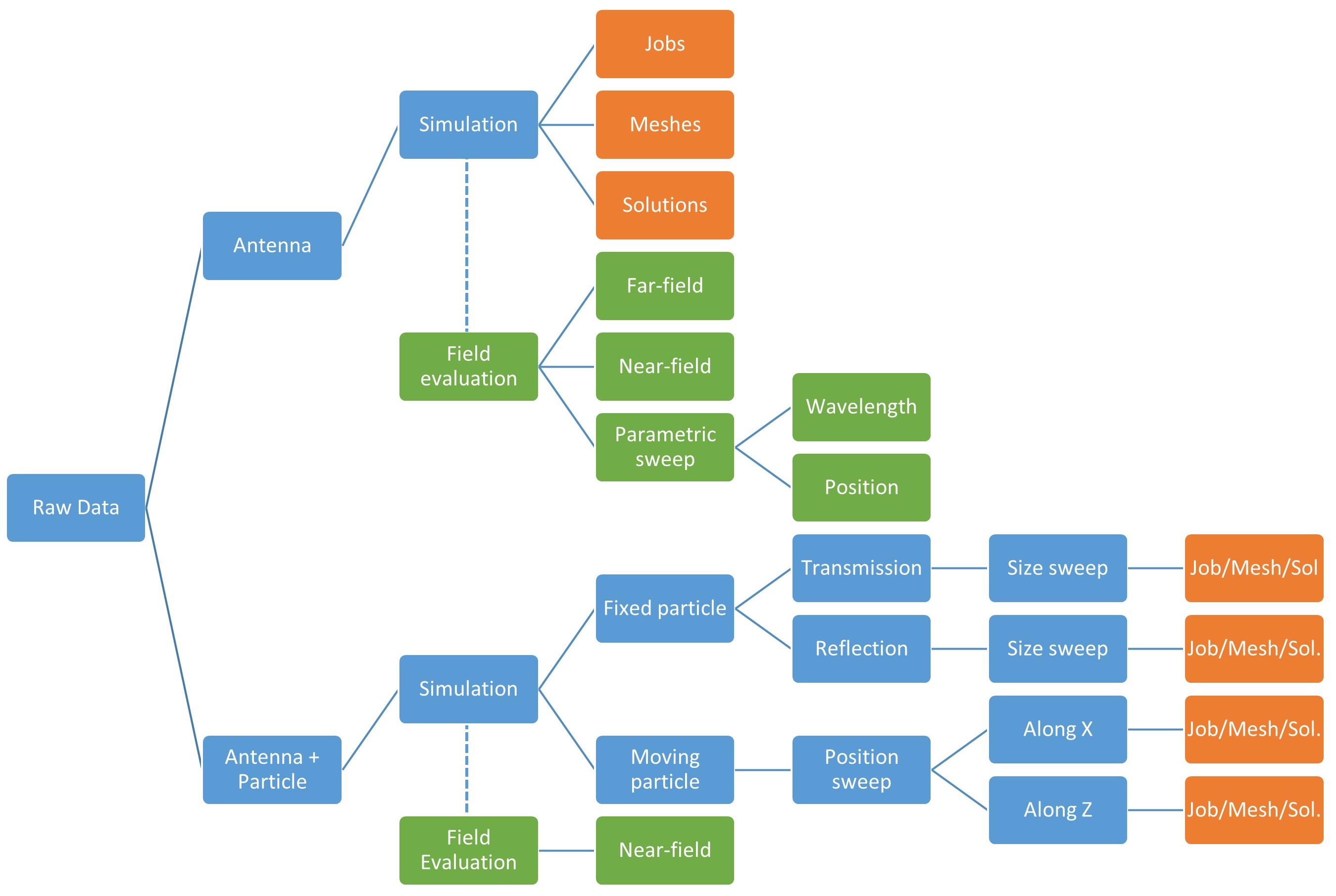
The image below shows the data structure inside the RawData folder. It gives a basic idea of how they are categorized.
1. Job file
A job file describes the input parameters set for a simulation. The job file is in the XML format, and it contains the following information.
- Simulation mesh
- Wavelength
- Material parameters of different simulation domains
- Illumination parameters
Using the cell below, you can check the content of a job file. You should set a proper file location in the following cell. You can also open the .xml file directly in job folders.
import pandas as pd
import xml.etree.ElementTree as ET

job_file = 'RawData\Antenna\Simulation\job\\29.xml'
tree = ET.parse(job_file)
root = tree.getroot()

for elem in root:
    print(' '.join(elem.tag.split())+":", ' '.join(elem.text.split()), end='\n')
    for subelem in elem:
        print('\t'+' '.join(subelem.tag.split())+":", subelem.text)
In a surface integral equation (SIE) formulation routine, the three-dimensional space is partitioned into domains defined by a common material (identical dielectric permittivity and magnetic permeability). The material parameters specified as nonperiodicdomain shows relative permittivities and relative permeabilities, i.e., (Re(eps), Im(eps)) (Re(mu), Im(mu)) of a domain. Each of them is index by an integer 0, 1, 2 …. You can check the domain index in the simulation mesh.
The illumination part consists of three parameters: 1) the domain index of the incident wave, 2) the propagation direction, and 3) the complex polarization in a three-dimensional Cartesian coordinate system, (x, y, z).
2. Simulation mesh
A surface mesh is a discrete approximation of the domains’ boundary surfaces. The surface mesh file of the standard type .mesh contains the necessary information to generate a surface mesh that will be used for the calculations. An example of a mesh looks like:
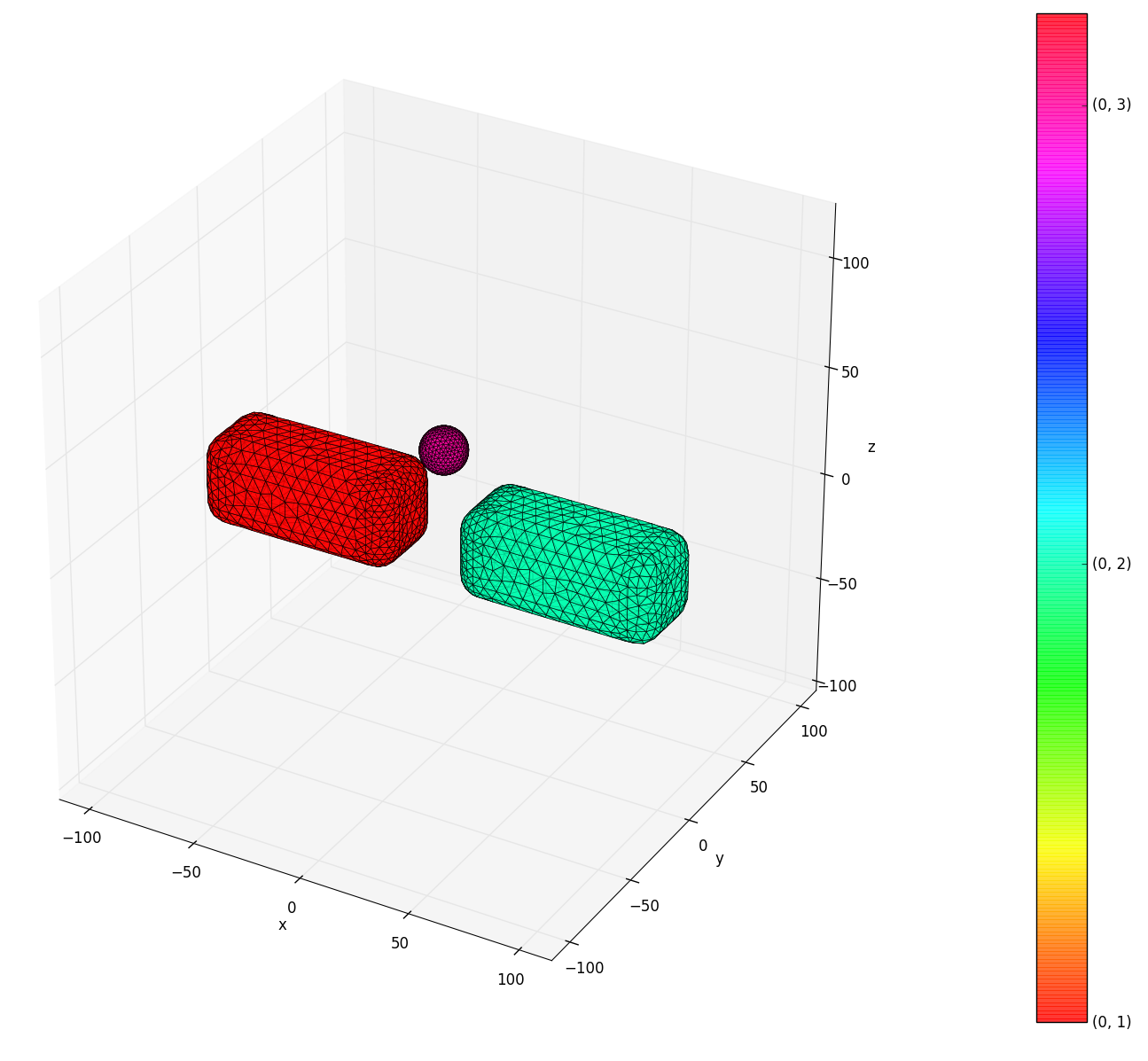
You can use python/meshviewer.py to visualize a mesh by yourself. (It's a Python 2 script.)
3. Solutions: Electric and magnetic surface currents
The SIE calculation gives electric and magnetic surface current densities as a solution. A typical solution file has J and M values for all edges created by the mesh file. The vectors J and M are the electric and magnetic surface current densities
df = pd.read_csv('RawData\Antenna\Simulation\solution\\0.sol',
                header=None)

df[0] = df[0].str.strip('\(')
df[1] = df[1].str.strip('\)')
df.columns = ['J', 'M']
df.index.name = 'Edges'
df.head()
It is difficult to get a physical insight directly from the vectors J and M. We can process these values to obtain electric and magnetic fields as in the following section, or we can use it directly to evaluate the Maxwell's stress tensor to compute the optical forces.
4. Obtaining electromagnetic fields from solutions
4-1. Defining points
From the surface current densities, we can evaluate the electric and magnetic fields at an arbitrary location. We use a file containing a set of points where we want to evaluate the fields. In a typical position file, each point is specified with the x, y, and z coordinates, as shown below.
points = pd.read_csv('RawData\Antenna\FieldEvaluation\\farfield\points',
                    sep='\s+',
                     header=None)
points.columns = ['x','y','z']
points.head()
The units are in nanometers (nm). This example of a point file has points over a sphere of 50 micron-radius. It is to evaluate electromagnetic far-fields for calculating scattering cross-sections.
import plotly.graph_objects as go
fig = go.Figure(data=[go.Scatter3d(x=points.x, y=points.y, z=points.z,
                                   mode='markers',
                                   marker=dict(
                                       size=3,
                                       color=points.z,                # set color to an array/list of desired values
                                       colorscale='Viridis',   # choose a colorscale
                                       opacity=0.5
                                   )
                                  )])
# tight layout
fig.update_layout(margin=dict(l=0, r=0, b=0, t=0))
fig.show()
4-2. Evaluating the incident and scattered fields
The complex fields E, B, D, and H are evaluated at each of these positions. Each of their components is given in a pair of real and imaginary parts in the x, y, and z directions. Each line in the field file corresponds to the position given in the positions file.
The incident field is stored in files ending with .ein and .hin, while the scattered field is stored in files ending with .esc and .hsc. The total field is the sum of the incident with the scattered field. The incident field is defined to have non-zero values only in the domain it is put.
ein = pd.read_csv('RawData\Antenna\FieldEvaluation\\farfield\\0.ein',
                 sep="\s+|,",
                 header=None,
                 engine="python")
ein.columns = ['Re($E_x$)','Im($E_x$)','Re($E_y$)','Im($E_y$)','Re($E_z$)','Im($E_z$)']
esc = pd.read_csv('RawData\Antenna\FieldEvaluation\\farfield\\0.esc',
                 sep="\s+|,",
                 header=None,
                 engine="python")
esc.columns = ['Re($E_x$)','Im($E_x$)','Re($E_y$)','Im($E_y$)','Re($E_z$)','Im($E_z$)']
ein.head()
esc.head()